Longitudinal data, or data collected multiple times from the same cases, are increasingly popular. They come in many shapes and sizes, from traditional panel surveys to social media, administrative, or sensor data. One of the great strengths of this type of data is its ability to facilitate causal analysis. While it does not “prove causality”, by understanding the causal order of events, we can get one step closer to understanding the underlying processes involved in the social world.
This type of data can also help answer one particular kind of question that appears in many fields: what is the causal direction of variables? For example, we might know that mental and physical health are related, but we might not be sure which is the cause and which is the effect. We may have plausible theoretical mechanisms in both directions. For example, a decrease in physical health can lead to anxiety, depression and outcomes associated with mental health. We can also think of an opposite process where a sudden reduction in mental health can lead to lower physical health due to a decrease in physical activity.
Longitudinal data can be used to disentangle such processes. One of the models developed explicitly to investigate such questions is the cross-lagged model. This model uses the Structural Equation Modelling (SEM) framework to estimate the two processes concurrently while controlling for possible confounders. In this blog post, we will walk through how to apply this method using R and how you can formally test the causal direction of two variables.
Want to really learn? Follow along using the data and code.
Get them when you join the newsletter. Additionally, you will get my 63-point pre-submission checklist for your research. All for free!
The cross-lagged model
To understand this model, we can use the SEM visualization framework. In this framework, observed variables are represented by squares, regression coefficients by single-headed arrows, correlations by double-headed arrows, and residuals by small circles.
Given this notation, we can represent the cross-lagged model using such a graph:
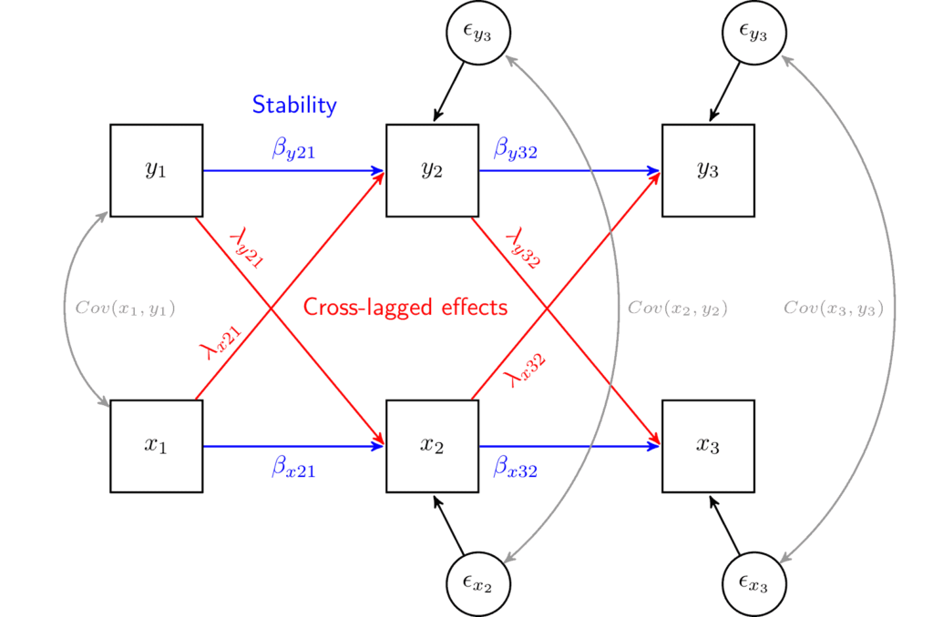
Here, we have two variables of interest: x and y. They are each measured at three points in time (e.g., x1, x2, x3). The model has three different parts:
- Cross-lagged effects capture the impact of one variable at a previous wave on another’s current values. For example, λy21 (lambda) represents the effect of y in wave 1 on x in wave 2. The opposite effect, λx21, represents the effect of x in wave 1 on y in wave 2. By comparing these two coefficients, we can understand if the effects in one direction are stronger than those in the other. This comparison is at the heart of this model and informs us about the causal direction.
- Stability coefficients capture how stable each variable is. It is estimated by including auto-regressive coefficients in which the values at the previous wave influence the values at the current wave. For example, coefficient βy21 (beta) captures the stability of y1 on y2. If y represents something like mental health, we would interpret it as the stability of mental health from wave 1 to wave 2. The closer the value is to 1, the more stable the variable (i.e., cases don’t change their rank order on mental health). If the coefficient is close to 0, it means that the previous values do not affect the current status, while if it is -1, it means that the order of the individuals on that variable is reversed. Typically, in this model, we are not interested in this type of coefficient, but we treat it as a control. We are effectively controlling for previous levels of x and y, which, in turn, makes the assumption of controlling for possible confounders more plausible. These coefficients are also known as lag-1 effects or a Markov chain, as the model implies that only the prior wave information is important for the current status.
- Time-specific correlations capture the correlation between the two variables of interest at each point in time. They also control possible time-specific confounders that might impact both variables. For example, a global pandemic may occur during the data collection at the second time point, leading to a decrease in both x and y. These correlations would capture this process and control for it.
We can also represent the model using a set of formulas. These represent the same model as above. The β coefficients represent the stability, and the λ represents the cross-lagged effects. The ϵ (epsilon) is each dependent variable’s regression residual coefficients (or unexplained variance). The ν (nu) represents the intercept or the expected value of the outcome when the predictors are 0. Lastly, we correlate x and y at each wave (j).
xj = νxj + βx, j, j − 1xj − 1 + λy, j, j − 1yj − 1 + ϵxj
yj = νyj + βy, j, j − 1yj − 1 + λx, j, j − 1xj − 1 + ϵyj
Cov(xj,yj)
Running the cross-lagged model in R
Now that we have an idea about why we would use the cross-lagged model and its main components, we can see how to estimate it in R. Here, we will use data from the first three waves of the Understanding Society survey. Our research question focuses on the causal direction of mental health (“mcsc”) and physical health (“pcsc”). These are calculated scores based on the SF12 scale. The values go from 0 to 100, where a higher number = better health.
Here, we centred the variables. We do this by subtracting the average from each variable, so the new mean is 0. This does not change regression coefficients but does make intercepts easier to interpret.
To run the model, we use the lavaan package.
library(tidyverse)
library(lavaan)

load("./data/us_clean_syn.RData")

usw <- usw |>
  mutate(
    pcsc_1 = sf12pcs_1 - mean(sf12pcs_1, na.rm = TRUE),
    pcsc_2 = sf12pcs_2 - mean(sf12pcs_2, na.rm = TRUE),
    pcsc_3 = sf12pcs_3 - mean(sf12pcs_3, na.rm = TRUE),
    mcsc_1 = sf12mcs_1 - mean(sf12mcs_1, na.rm = TRUE),
    mcsc_2 = sf12mcs_2 - mean(sf12mcs_2, na.rm = TRUE),
    mcsc_3 = sf12mcs_3 - mean(sf12mcs_3, na.rm = TRUE)
  )
We split the process into three steps. First, we write the model as a simple text object and save it as “model”:
model <- 'pcsc_2 ~ 1 + pcsc_1 + mcsc_1
          pcsc_3 ~ 1 + pcsc_2 + mcsc_2

          mcsc_2 ~ 1 + mcsc_1 + pcsc_1
          mcsc_3 ~ 1 + mcsc_2 + pcsc_2

          pcsc_1 ~~ mcsc_1
          pcsc_2 ~~ mcsc_2
          pcsc_3 ~~ mcsc_3'
We have four regression models represented by the “~” symbol. We have the dependent variable or outcome on the left of the symbol. On the right side, we have the predictors or independent variables. For example, the first line says that we want to explain physical health in wave 2 (“pcsc_2”) by physical health in wave 1 (“pcsc_1”, this represents stability) and mental health in wave 1 (“mcsc_1”, this represents the cross-lagged effect). The “1” value in the regression represents the intercept. We also include correlations between variables at each wave, represented by ~~.
Note that lavaan figures out if the correlation is between the observed variables or the residuals.
Now that we have the model, we can estimate it using the sem() command. We give it as inputs the model and the data (“usw” stands for Understanding Society in wide format). We also add an option to estimate the model using Full Information Maximum Likelihood (missing = "ML"). This uses all the available information to estimate the model and leads to fewer missing cases in the model than listwise deletion (which is the default).
m1 <- sem(model, data = usw, missing = "ML")
Now that the model is stored as “m1”, we can print the results using the summary() command. We also ask for the standardized coefficients using the standardized = TRUE option.
summary(m1, standardized = TRUE)
## lavaan 0.6-19 ended normally after 91 iterations
##
##   Estimator                                         ML
##   Optimization method                           NLMINB
##   Number of model parameters                        23
##
##                                                   Used       Total
##   Number of observations                         48440       51007
##   Number of missing patterns                         7
##
## Model Test User Model:
##
##   Test statistic                              5063.374
##   Degrees of freedom                                 4
##   P-value (Chi-square)                           0.000
##
## Parameter Estimates:
##
##   Standard errors                             Standard
##   Information                                 Observed
##   Observed information based on                Hessian
##
## Regressions:
##                    Estimate  Std.Err  z-value  P(>|z|)   Std.lv  Std.all
##   pcsc_2 ~
##     pcsc_1            0.607    0.005  128.736    0.000    0.607    0.618
##     mcsc_1            0.102    0.005   18.908    0.000    0.102    0.091
##   pcsc_3 ~
##     pcsc_2            0.570    0.005  107.215    0.000    0.570    0.583
##     mcsc_2            0.079    0.006   12.413    0.000    0.079    0.070
##   mcsc_2 ~
##     mcsc_1            0.290    0.006   51.353    0.000    0.290    0.302
##     pcsc_1            0.036    0.005    7.095    0.000    0.036    0.042
##   mcsc_3 ~
##     mcsc_2            0.452    0.006   75.997    0.000    0.452    0.457
##     pcsc_2            0.069    0.005   13.154    0.000    0.069    0.081
##
## Covariances:
##                    Estimate  Std.Err  z-value  P(>|z|)   Std.lv  Std.all
##   pcsc_1 ~~
##     mcsc_1            0.795    0.535    1.485    0.138    0.795    0.007
##  .pcsc_2 ~~
##    .mcsc_2          -10.064    0.496  -20.279    0.000  -10.064   -0.123
##  .pcsc_3 ~~
##    .mcsc_3          -15.103    0.498  -30.304    0.000  -15.103   -0.197
##
## Intercepts:
##                    Estimate  Std.Err  z-value  P(>|z|)   Std.lv  Std.all
##    .pcsc_2           -0.391    0.052   -7.503    0.000   -0.391   -0.035
##    .pcsc_3           -0.111    0.056   -1.983    0.047   -0.111   -0.010
##    .mcsc_2           -0.265    0.055   -4.812    0.000   -0.265   -0.027
##    .mcsc_3            0.015    0.053    0.275    0.783    0.015    0.002
##     pcsc_1           -0.024    0.053   -0.458    0.647   -0.024   -0.002
##     mcsc_1           -0.004    0.046   -0.077    0.938   -0.004   -0.000
##
## Variances:
##                    Estimate  Std.Err  z-value  P(>|z|)   Std.lv  Std.all
##    .pcsc_2           77.832    0.662  117.539    0.000   77.832    0.610
##    .pcsc_3           80.159    0.726  110.466    0.000   80.159    0.658
##    .mcsc_2           86.335    0.734  117.594    0.000   86.335    0.907
##    .mcsc_3           73.169    0.662  110.468    0.000   73.169    0.787
##     pcsc_1          132.207    0.859  153.861    0.000  132.207    1.000
##     mcsc_1          102.607    0.666  153.978    0.000  102.607    1.000
The coefficients of interest are under the “Regressions” section of the output. Physical health has stability coefficients of 0.607 and 0.570, while the corresponding mental-health coefficients are 0.290 and 0.452. The outcomes therefore remain related to their earlier values, although the estimates are smaller than those in the previous output.
The cross-lagged effects from mental health to later physical health are 0.102 and 0.079. The corresponding effects from physical health to later mental health are 0.036 and 0.069. All four effects are statistically different from zero. As before, the results suggest reciprocal relationships, with the mental-to-physical paths somewhat larger at both transitions.
To help interpret this model, I recommend drawing the model and adding the observed coefficients in the appropriate place. For example, if we take the coefficients from the output and put them in the SEM figure, we would get:

The graph shows that mental and physical health are related in both directions. The mental-to-physical effect is larger at each transition. Next, we can test formally whether the two coefficients at the first transition differ significantly.
Note that here, the two variables use the same scale, and we can compare them using the unstandardized coefficients. When the variables have different scales, either rescale them or interpret the standardized coefficients (the last column in the output “Std.all”).
Testing the equality of cross-lagged coefficients
The SEM framework offers some useful tools for explicitly testing the equality of coefficients. The typical procedure for this is to run a model without constraints (like the one we ran above) and then run a model with some constraints. These can be added by fixing a coefficient to a particular value (e.g., saying a regression coefficient is 0) or forcing some coefficients to be equal.
Our research question focuses on the equality of the cross-lagged effects. We want to formally test if the impact of mental health on physical health is significantly different from the reverse relationship. Adding such a restriction gives the two coefficients the same “name.” Below is a visual representation where we show how we would restrict the cross-lagged effects from wave 1 to wave 2 to be called “a” while those from wave 2 to wave 3 to be called “b.”
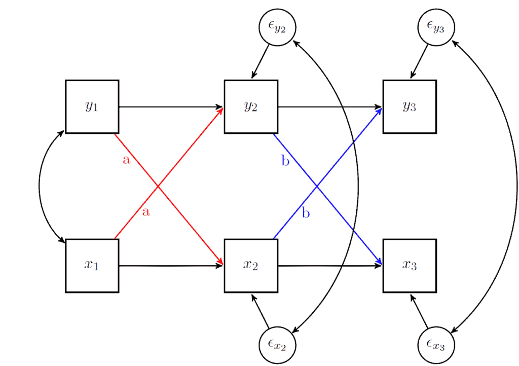
In general, I recommend doing this in stages. Here, we test whether the cross-lagged coefficients from wave 1 to wave 2 are equal. This compares 0.102 with 0.036 in the population. If the restricted model fits significantly worse, we can conclude that the two effects differ.
To add a name or a restriction in lavaan we simply put the value before the coefficient with a “*” next to it. The code below fixes the cross-lagged coefficients from wave 1 to wave 2 to be called “a” (thus making them equal).
model <- 'pcsc_2 ~ 1 + pcsc_1 + a*mcsc_1
          pcsc_3 ~ 1 + pcsc_2 + mcsc_2

          mcsc_2 ~ 1 + mcsc_1 + a*pcsc_1
          mcsc_3 ~ 1 + mcsc_2 + pcsc_2

          pcsc_1 ~~ mcsc_1
          pcsc_2 ~~ mcsc_2
          pcsc_3 ~~ mcsc_3'

m2 <- sem(model, data = usw, missing = "ML")

summary(m2, standardized = TRUE)

## lavaan 0.6-19 ended normally after 92 iterations
##
##   Estimator                                         ML
##   Optimization method                           NLMINB
##   Number of model parameters                        23
##   Number of equality constraints                     1
##
##                                                   Used       Total
##   Number of observations                         48440       51007
##   Number of missing patterns                         7
##
## Model Test User Model:
##
##   Test statistic                              5142.904
##   Degrees of freedom                                 5
##   P-value (Chi-square)                           0.000
##
## Parameter Estimates:
##
##   Standard errors                             Standard
##   Information                                 Observed
##   Observed information based on                Hessian
##
## Regressions:
##                    Estimate  Std.Err  z-value  P(>|z|)   Std.lv  Std.all
##   pcsc_2 ~
##     pcsc_1            0.603    0.005  128.335    0.000    0.603    0.616
##     mcsc_1     (a)    0.066    0.004   18.166    0.000    0.066    0.060
##   pcsc_3 ~
##     pcsc_2            0.570    0.005  107.139    0.000    0.570    0.581
##     mcsc_2            0.083    0.006   13.141    0.000    0.083    0.074
##   mcsc_2 ~
##     mcsc_1            0.296    0.006   52.594    0.000    0.296    0.306
##     pcsc_1     (a)    0.066    0.004   18.166    0.000    0.066    0.078
##   mcsc_3 ~
##     mcsc_2            0.451    0.006   76.022    0.000    0.451    0.458
##     pcsc_2            0.065    0.005   12.415    0.000    0.065    0.076
##
## Covariances:
##                    Estimate  Std.Err  z-value  P(>|z|)   Std.lv  Std.all
##   pcsc_1 ~~
##     mcsc_1            0.775    0.535    1.447    0.148    0.775    0.007
##  .pcsc_2 ~~
##    .mcsc_2          -10.088    0.498  -20.277    0.000  -10.088   -0.123
##  .pcsc_3 ~~
##    .mcsc_3          -15.105    0.498  -30.301    0.000  -15.105   -0.197
##
## Intercepts:
##                    Estimate  Std.Err  z-value  P(>|z|)   Std.lv  Std.all
##    .pcsc_2           -0.372    0.052   -7.138    0.000   -0.372   -0.033
##    .pcsc_3           -0.116    0.056   -2.070    0.038   -0.116   -0.011
##    .mcsc_2           -0.282    0.055   -5.128    0.000   -0.282   -0.029
##    .mcsc_3            0.019    0.053    0.365    0.715    0.019    0.002
##     pcsc_1           -0.024    0.053   -0.462    0.644   -0.024   -0.002
##     mcsc_1           -0.002    0.046   -0.051    0.959   -0.002   -0.000
##
## Variances:
##                    Estimate  Std.Err  z-value  P(>|z|)   Std.lv  Std.all
##    .pcsc_2           77.904    0.663  117.500    0.000   77.904    0.616
##    .pcsc_3           80.173    0.726  110.454    0.000   80.173    0.659
##    .mcsc_2           86.487    0.736  117.486    0.000   86.487    0.900
##    .mcsc_3           73.171    0.662  110.467    0.000   73.171    0.786
##     pcsc_1          132.208    0.859  153.865    0.000  132.208    1.000
##     mcsc_1          102.603    0.666  153.983    0.000  102.603    1.000
In the restricted model, the two coefficients named “a” have the same value: 0.066. We can now compare this model with the previous one to see whether the equality restriction makes the fit worse.
There are different ways to compare models in SEM. A quick way to do it is to use the anova() command with the two models we estimated. This will create a small table with the AIC, BIC and the Chi-square test for the difference:
anova(m1, m2)

##
## Chi-Squared Difference Test
##
##    Df     AIC     BIC  Chisq Chisq diff    RMSEA Df diff Pr(>Chisq)
## m1  4 1516407 1516609 5063.4
## m2  5 1516485 1516678 5142.9      79.53 0.040264       1  < 2.2e-16 ***
## ---
## Signif. codes:  0 '***' 0.001 '**' 0.01 '*' 0.05 '.' 0.1 ' ' 1
AIC and BIC are relative fit indices. They do not have a fixed scale, but lower values are better. Based on these two indicators, “m1” is better. We can also use the Chi-square difference test (sometimes represented as Δχ2). This takes the difference of the Chi-square and the degrees of freedom of the two models. The null hypothesis is that the models have equal fit. Here, the test is statistically significant. This implies that the model with the restriction (“m2”) is significantly worse than the first model. As a result, we should select “m1”.
All the fit indices favour “m1”. The chi-square difference is 79.53 with one degree of freedom (p < .001). We therefore reject the equality restriction and conclude that the mental-to-physical effect of 0.102 is larger than the physical-to-mental effect of 0.036.
We should still be careful when interpreting this comparison. Both cross-lagged coefficients are statistically different from zero, so the results support influence in both directions. Their difference is 0.066 (0.102 − 0.036). Whether this is substantively important depends on the research context, theory and existing evidence.
Want to really learn? Follow along using the data and code.
Get them when you join the newsletter. Additionally, you will get my 63-point pre-submission checklist for your research. All for free!
Conclusions
We saw how we can use longitudinal data and the cross-lagged model to understand the causal direction of two variables. This model is useful when we have two related variables but are unsure about the causal direction. We saw how we can run the model in R and lavaan and how we can formally test the equality of the coefficients.
The model represents an elegant way to test the causal direction. It also has the advantage of controlling for some possible confounders. This is done by controlling for the values on the variables of interest at the previous wave (i.e., the stability coefficients) and with the time-specific correlations. That being said, the model is far from perfect. It is still possible to have missing confounders that could bias our estimates (which we might want to control for). You can see how to include controls in this blog post. Also, in this form, the model does not separate “within” and “between” variation (see this post for a discussion on these two types of variance). The SEM framework is extremely flexible, and the model can be extended to deal with these challenges.
For more on longitudinal data analysis, check out an introduction to the multilevel model for change and one for the latent growth model.
Want to take your skills to the next level? Join our next live course to learn how to efficiently prepare and explore data as well as the main frameworks for analysing longitudinal data.