Longitudinal data analysis often involves complex processes, including data preparation, cleaning, modeling, and presentation. As a result, having a clear and structured workflow is essential. A good workflow ensures that the analysis is reproducible, transferable, and easy to revise and share. Without a structured approach, it is easy to lose track of decisions and steps, leading to confusion or errors.

Here are some key principles to consider when developing your data workflow:

• No copy and paste: Avoid manual copying and pasting. Instead, write scripts that automate repetitive tasks to ensure consistency and reduce errors. When coding, an useful rule of thumb is to not copy and edit a piece of code more than twice. If you are doing repetitive coding it may be better to write a function or a loop instead. Also, never copy and paste results as this is prone to errors and cannot be easily replicated.
• Back up your work: Always back up your scripts and data. A simple way to do that is by using a service like Dropbox or One drive. Even better, using a version control system like Git makes it possible to create a full history of the documents you worked on. By combining Git with GitHub, you can back up your work in the cloud and make it available publicly or with a smaller group of collaborators (more on this below).
• Document your work: Document your code, decisions and workflow. Use comments in your scripts and commit messages in version control systems to explain what and why you are doing something. While this might be obvious at the time it will be less so for your colleagues and even for yourself in the future.
• Make your work transferable: Use tools like relative paths, dynamic documents, and self-contained project structures to ensure that your analysis can run seamlessly on another system. This is especially important if you are collaborating with others or planning to share your work.

Using version control with Git and GitHub for reproducible workflows

Git is a powerful version control system that creates a history of your work as well as associated documentation for each important step. It also facilitates collaboration with others. You can also combine Git with GitHub, facilitating online back-ups and collaboration with others.

The main strengths of version control software such as Git (+ GitHub):

• Version control: Track changes to your project files over time, allowing you to revert to previous versions if needed.
• Collaboration: Work with others on the same project and manage version conflicts.
• Backup: Store your project in the cloud, ensuring that your work is safe and accessible.
• Documentation: Keep a clear history of your project, including who made changes and why.
• Branches: Work on different features or analyses simultaneously without affecting the main project.

Git works by creating a local repository that stores your project files and their history. You can then commit changes to the repository, creating a snapshot of your work at that point in time. By using branches, you can work on different features or analyses simultaneously without affecting the main project. When you are ready, you can merge these branches back into the main project.

Git and GitHub are well integrated in RStudio, making it easy to manage your project. Once you install Git on your computer you can get started by initializing a Git repository in your project directory:

usethis::use_git()

Alternatively you can also initialize a Git repository from the menu options in RStudio or when you create an Rstudio project.

After you did some work in the project and are at a stage where you want to save what you have done you can do a commit. When you commit you need to decide the changes you want to save and add a comment that explains what you have done. You can commit them to the repository using using the Rstudio menu or a command such as:

usethis::use_git_commit("Description of changes")

Committing is a process that happens locally, on your computer. If you want to backup your work on GitHub the next step would be to push the changes to the remote repository (you first need to create a GitHub account and link it to RStudio). You can do this using the RStudio menu or the following command (or using the Rstudio menu):

usethis::pr_push()

Pushing sends the current code to the remote repository on GitHub. This is useful if you want to share your work with others or if you want to have a backup of your work in the cloud.

The opposite of pushing is pulling. Pulling is used to get the latest version from the remote repository. This is useful if you are working with others and want to incorporate their changes into your work. You can pull changes using the RStudio menu or the following command:

usethis::pr_pull()

These are just some of the basics of Git and GitHub. There are many more features and commands that can be used to manage your project. Keep in mind that there is some initial work to set up Git and GitHub properly and to link it to RStudio. For a more detailed introduction to Git and GitHub you can check out the online book Happy Git with R.

Managing dependencies in R with the renv package

Often we work on multiple projects at different points in time. As R and packages change it may become difficult to reproduce results or to re-run code from the past. The R package renv partially solves this problem. It does this by installing and managing separate packages for each project. By creating a local library of packages for your project, renv ensures that the same versions of packages are used regardless of when or where the analysis is run. This is especially useful for complex projects that might span over months or years.

You can activate renv when creating a new project in RStudio. Alternatively, you can also initialize it in an existing project directory:

renv::init()

This creates a snapshot of your current package environment. You can restore this environment later with:

renv::restore()

Now, when you install packages they will be installed directly in the project folder. When you open you RStudio project again it will automatically load the local packages. This makes it easier to share your project with others or to run it on a different computer. This is also very useful if you need to go back to an old project and rerun the analysis (e.g., to revise a paper). The package will also remember the version of R you used and make it possible to restore all the packages you used in the past (e.g., if these were deleted), again helping reproduce your results.

Structuring projects and using relative paths

Another aspect to consider when working on more complex projects is how to organize your folders. Consider the following folder structure as a way to organize your longitudinal data projects:

project/
├── data/
├── scripts/
├── results/
├── figures/
└── reports/

• data: Store raw and cleaned datasets here
• scripts: Add your R scripts here. If the project is more complex separate your scripts by stage (e.g., cleaning, analysis, visualization)
• results: Save intermediate outputs like model results, estimates and tables
• figures: Keep all visualizations and graphs in one place
• reports: Use dynamic documents (e.g., R Markdown) to generate reports that combine text, code, and results (more below)

Of course, you can adapt this structure your needs. Other useful folders that you might want to consider are: “documentation” (e.g., for the data used), “literature” (for papers and references), “presentations” (for slides and presentations), and “manuscript” (for versions of a paper).

Another good practice is the use of “relative” as opposed to “absolute” paths. An absolute path shows where to find a file on the computer and looks like “C:/Users/YourName/project/data/your_dataset.csv” (for a Windows computer). The disadvantage of this approach is that the code will not work if you move the project somewhere else or if a collaborator tries to run your code on a different device.

An alternative to this is to use a relative path, such as “data/your_dataset.csv”. This path is relative to your working directory. If you use a Rstudio project it will automatically set the working directory to your project folder. In this way the path will work regardless of where the project is stored. For example, you can read a dataset using a relative path like this (i.e., file “your_dataset.csv” from the “data” subfolder):

read.csv("data/your_dataset.csv")

Now, once you set up the working directory (or if you use an RStudio project) you can use relative paths to access files in your project. This makes it easy to run code across multiple devices.

Also try to have a consistent naming convention. In general try to avoid having spaces in the names of folders or files as it sometimes leads to confusion. So use a folder name like “raw_data” instead of “raw data”. I also tend to use only lower case in my naming convention to avoid confusion but this is more of a personal preference.

Stages of a workflow

So, given these principles and tools, what does a typical workflow for longitudinal data analysis look like? Here are some steps to consider:

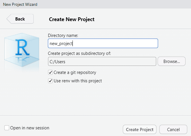
1. Set up the project: Create a folder for the project, set-up the working directory, initiate a Git repository and activate renv. All of this can be done easily in RStudio by creating a “New Project” (remember to select to initiate a Git repository and renv in the menu).

2. Create a project structure: Decide what kind of files you will be working with and create a folder structure that makes sense for your project. This can include folders for data, scripts, results, figures, and reports. This can be done in the “Files” pane in RStudio or by using commands (that need to be run only once) such as:

dir.create("data")
dir.create("scripts")
dir.create("results")
dir.create("figures")
dir.create("reports")

3. Data preparation: Often this is one of the most time consuming parts of working with data. Write scripts for importing, cleaning, and reshaping your data. If the scripts become long separate each step in different scripts to make the process more modular. Also, consider numbering the scripts so it is clear in which order they should be run (e.g., “01_data_import.R”, “02_data_clean.R”, etc.). Ideally each script should have a clear set of inputs and outputs and all of them should be run to create the final results of your analysis.
4. Analysis: Again, create scripts for doing the analysis. When conducting more complex analyses consider separate scripts for exploratory analysis, model fitting, and presenting of results.
5. Reports and presentations: Use dynamic documents (e.g., R Markdown or Quarto) to create reproducible reports or presentations to share with others.
6. Work in stages: Try to divide your work in stages. A stage could be when you finished doing something in R, for example finished the data cleaning, the analysis, a report, etc. You can also use the end of the coding session as a milestone. At this points commit your code to Git with a comment about what you have done in this stage. This will build a history of your work and make it easier to track changes.
7. Collaboration: If you are working with others, make sure to communicate about the workflow and the tools you are using. This will make it easier to collaborate and avoid confusion. Consider using GitHub as a tool for collaboration and sharing your work. If you do use GitHub remember to start your work session by Pulling the latest version of the code and end it by Pushing your changes.

Conclusions

By following these steps and principles, you can create an efficient, reproducible workflow for longitudinal data analysis. A well-structured workflow is not just about organization—it’s about ensuring that your findings are robust, your process is transparent, and your work can be easily shared and built upon by others.

Also keep in mind that it takes time to learn all of these tools and to develop a workflow that works for you. That being said, it is worth the investment as it will save you time in the long run and make your work more efficient and reproducible.

To learn how these practices fit in the larger workflow you need to follow when working with longitudinal data check out this post. You can also check out how to use dynamic documents here and how to present results here.

---