In a previous post, we introduced the multilevel model for change, a powerful model that can estimate change in time while separating within and between variation. While we discussed the basic model in detail, it can be expanded in several ways. Here, we will cover how to estimate non-linear change in time using the multilevel framework.
In the basic multilevel model for change, we have only one coefficient to describe the effect of time. This implies a stable or linear rate of change. In many applications, this is not an appropriate assumption, as rates of change can be different at different points in time. There are two main ways of modelling these non-linear trends: including polynomials and treating time as discrete.
Want to really learn? Follow along using the data and code.
Get them when you join the newsletter. Additionally, you will get my 63-point pre-submission checklist for your research. All for free!
Nonlinear change in time using polynomials
Let’s start with the first approach, including polynomials of time in the model. This is quickly done by creating new variables that take the values of time and square/cube/etc them. We will use as reference “wave0” which is a recoded version of time that starts from 0 (this is used to make the intercept easier to interpret, as discussed here).
library(tidyverse)
library(lme4)

load("./data/usl_all_syn.RData")

complete_ids <- usl_all |>
  filter(wave <= 6) |>
  group_by(pidp) |>
  summarise(
    complete = n() == 6 && all(!is.na(logincome)),
    .groups = "drop"
  ) |>
  filter(complete) |>
  pull(pidp)

usl <- usl_all |>
  filter(pidp %in% complete_ids, wave <= 6)

usl <- mutate(
  usl,
  wave0 = wave - 1,
  wave_sq = wave0^2,
  wave_cu = wave0^3
)

select(usl, wave0, wave_sq, wave_cu)
## # A tibble: 127,068 × 3 ## wave0 wave_sq wave_cu ## <dbl> <dbl> <dbl> ## 1 0 0 0 ## 2 1 1 1 ## 3 2 4 8 ## 4 3 9 27 ## 5 4 16 64 ## 6 5 25 125 ## 7 0 0 0 ## 8 1 1 1 ## 9 2 4 8 ## 10 3 9 27 ## # ℹ 127,058 more rows
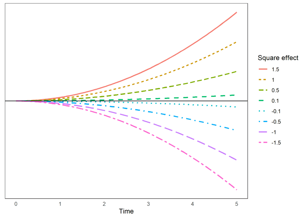
By including these new variables in a model, we allow for the effect of time to shift. When time has low values the main effect will have a large impact on the outcome, as time increases the square and the cube will become more and more important (due to their increased size). This allows for the rate of change to be different at different points in time. With the addition of each polynomial, we allow the change rate to “bend” once. If the effect of the polynomial is positive, the bend will be upwards, if it’s negative, it will bend downwards. The larger the size, the stronger the shift. Let’s look at an example. Below are the predicted scores for a hypothetical outcome where the main effect is 0. We see how the size of the outcome changes in time non-linearly due to the impact of the square estimate:
We can also look at some hypothetical examples that include a cube effect. Again, the main effect is 0, so it would indicate no trend. However, the combination of square and cube effects allows for different trends in time.
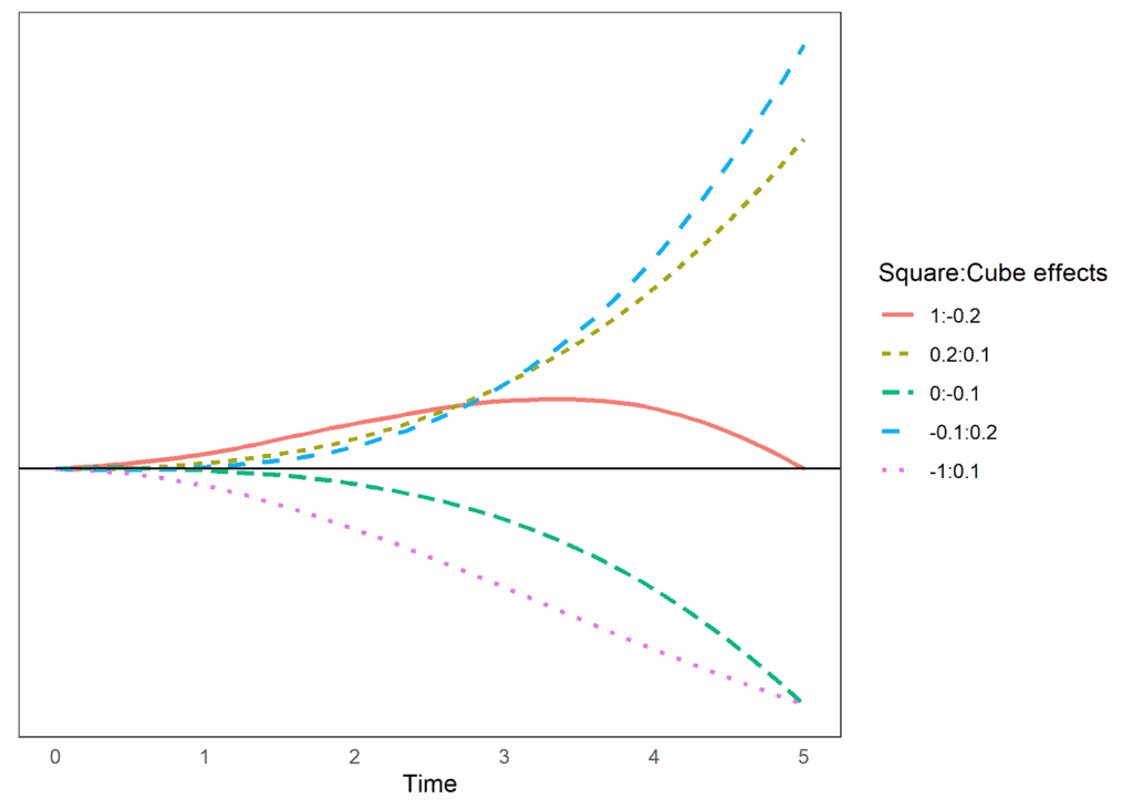
If we look at the situation when the square effect is 1, and the cube has an effect of -0.2, we see an initial upward trend and then a decrease, reaching 0 by wave 5. If both the square and the cube are positive, we will see an accelerated trend that increases as time passes. We also see that we can reach similar estimates in wave 5 with different change patterns. For example, both having a square effect of -1 and a cube effect of 0.1 and having a square effect of 0 and a cube effect of -.1 reach a similar point in wave 5, but if we continue that trend, the trajectories would become quite different.
Let’s look at the linear model so we can use it as a reference (for an in-depth interpretation of the coefficient, check this post).
model_control <- lmerControl(
  optimizer = "bobyqa",
  optCtrl = list(maxfun = 200000)
)

m2 <- lmer(
  data = usl,
  logincome ~ 1 + wave0 + (1 + wave0 | pidp),
  control = model_control
)

summary(m2)
## Linear mixed model fit by REML ['lmerMod']
## Formula: logincome ~ 1 + wave0 + (1 + wave0 | pidp)
##    Data: usl
## Control: model_control
##
## REML criterion at convergence: 343010
##
## Scaled residuals:
##     Min      1Q  Median      3Q     Max
## -7.3188 -0.1576  0.0694  0.2929  5.3691
##
## Random effects:
##  Groups   Name        Variance Std.Dev. Corr
##  pidp     (Intercept) 1.29501  1.1380
##           wave0       0.02997  0.1731   -0.64
##  Residual             0.52694  0.7259
## Number of obs: 127068, groups:  pidp, 21178
##
## Fixed effects:
##             Estimate Std. Error t value
## (Intercept) 6.873652   0.008613   798.1
## wave0       0.058614   0.001684    34.8
##
## Correlation of Fixed Effects:
##       (Intr)
## wave0 -0.656
These results imply that log income increases linearly by 0.059 for each wave. We can add polynomials if we believe the rate of change is not constant. For example, we can include the square of time using this code:
m2_sq <- lmer(
  data = usl,
  logincome ~ 1 + wave0 + wave_sq + (1 + wave0 | pidp),
  control = model_control
)

summary(m2_sq)
## Linear mixed model fit by REML ['lmerMod']
## Formula: logincome ~ 1 + wave0 + wave_sq + (1 + wave0 | pidp)
##    Data: usl
## Control: model_control
##
## REML criterion at convergence: 342930.4
##
## Scaled residuals:
##     Min      1Q  Median      3Q     Max
## -7.3515 -0.1582  0.0704  0.2932  5.3437
##
## Random effects:
##  Groups   Name        Variance Std.Dev. Corr
##  pidp     (Intercept) 1.2953   1.1381
##           wave0       0.0300   0.1732   -0.64
##  Residual             0.5264   0.7255
## Number of obs: 127068, groups:  pidp, 21178
##
## Fixed effects:
##               Estimate Std. Error t value
## (Intercept)  6.8475608  0.0090321 758.135
## wave0        0.0977514  0.0044137  22.147
## wave_sq     -0.0078274  0.0008159  -9.593
##
## Correlation of Fixed Effects:
##         (Intr) wave0
## wave0   -0.517
## wave_sq  0.301 -0.924
The quadratic model has an initial positive slope of 0.098 and a negative square effect of -0.008. We therefore expect log income to increase initially, with the rate of increase becoming smaller in later waves.
We can also compare the predicted scores from the model that assumes linear change and the model that also includes square effects against the observed average. It appears that the square effect fits the observed data better, albeit not perfectly.

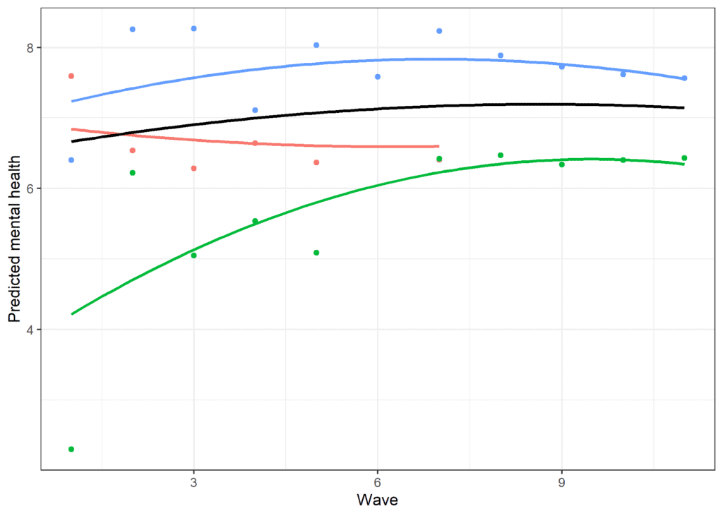
The previous model keeps the quadratic bend fixed across respondents. We can allow each respondent to have their own non-linear trajectory by adding the squared time term to the random part. The synthetic file provides all eleven waves for this example. We scale time only inside the random-effects terms to improve numerical estimation; the fixed effects remain on the original per-wave scale.
usl_all <- usl_all |>
  mutate(
    wave0 = wave - 1,
    wave_sq = wave0^2,
    wave_re = wave0 / 10,
    wave_sq_re = wave_re^2
  )

m2_sq_re <- lmer(
  data = usl_all,
  logincome ~ 1 + wave0 + wave_sq +
    (1 + wave_re + wave_sq_re | pidp),
  control = model_control
)

summary(m2_sq_re)
## Linear mixed model fit by REML ['lmerMod'] ## Formula: logincome ~ 1 + wave0 + wave_sq + (1 + wave_re + wave_sq_re | ## pidp) ## Data: usl_all ## Control: model_control ## ## REML criterion at convergence: 890416 ## ## Scaled residuals: ## Min 1Q Median 3Q Max ## -6.9844 -0.1506 0.0782 0.3077 4.9922 ## ## Random effects: ## Groups Name Variance Std.Dev. Corr ## pidp (Intercept) 1.6981 1.303 ## wave_re 9.8504 3.139 -0.64 ## wave_sq_re 7.4127 2.723 0.44 -0.91 ## Residual 0.6337 0.796 ## Number of obs: 307858, groups: pidp, 50994 ## ## Fixed effects: ## Estimate Std. Error t value ## (Intercept) 6.6540184 0.0064927 1024.84 ## wave0 0.1181185 0.0022988 51.38 ## wave_sq -0.0079764 0.0002315 -34.45
Across eleven waves, the model estimates an initial positive trend of 0.118 and a negative quadratic term of -0.008. We can see below the average change in time as well as three individuals with their trajectories.
Nonlinear change in time using a categorical variable
An alternative way to model non-linear change is to treat time as a discrete/categorical variable. In that case, we can estimate the expected value of the outcome at each point in time or in a particular range of time. The most general approach treats each time point as a discrete variable. While this doesn’t make any assumptions about the shape of the change in time, it is a complex model that may have estimation problems.
To try this out with our model, we can define the time variable as a factor. By default, lmer() (like the lm() command) transforms factors into dummy variables and treats the first category as the reference. We can use this to model non-linear change.
usl <- mutate(usl,
              wave_fct = as.factor(wave))
We can now include this in our model.
m2_dummy <- lmer(
  data = usl,
  logincome ~ 1 + wave_fct + (1 + wave0 | pidp),
  control = model_control
)

summary(m2_dummy)
## Linear mixed model fit by REML ['lmerMod']
## Formula: logincome ~ 1 + wave_fct + (1 + wave0 | pidp)
##    Data: usl
## Control: model_control
##
## REML criterion at convergence: 342809.3
##
## Scaled residuals:
##     Min      1Q  Median      3Q     Max
## -7.3267 -0.1602  0.0700  0.2944  5.3225
##
## Random effects:
##  Groups   Name        Variance Std.Dev. Corr
##  pidp     (Intercept) 1.29574  1.1383
##           wave0       0.03005  0.1733   -0.64
##  Residual             0.52553  0.7249
## Number of obs: 127068, groups:  pidp, 21178
##
## Fixed effects:
##             Estimate Std. Error t value
## (Intercept) 6.825304   0.009274  736.00
## wave_fct2   0.143486   0.007145   20.08
## wave_fct3   0.205471   0.007437   27.63
## wave_fct4   0.222739   0.007899   28.20
## wave_fct5   0.261674   0.008505   30.77
## wave_fct6   0.335933   0.009225   36.42
##
## Correlation of Fixed Effects:
##           (Intr) wv_fc2 wv_fc3 wv_fc4 wv_fc5
## wave_fct2 -0.465
## wave_fct3 -0.533  0.520
## wave_fct4 -0.583  0.515  0.567
## wave_fct5 -0.617  0.502  0.572  0.623
## wave_fct6 -0.639  0.484  0.569  0.633  0.678
Notice that we still treat the random part of the model linearly. Again, estimating a random effect at each wave can lead to issues with model estimation, so we use a simplified random effect.
The intercept gives the expected log income at wave 1, which is 6.825. At wave 2, the expected value is 6.825 + 0.143 = 6.969. The corresponding differences for waves 3 to 6 are 0.205, 0.223, 0.262 and 0.336. We can compare these values with the observed averages and the predictions from the quadratic model.

The new prediction is almost identical to the observed data (lines overlap). That being said, there is a trade-off between the model’s simplicity and how well it explains the data. We can formally compare the different models we estimated to decide how to treat the change in time for log income.
anova(m2, m2_sq, m2_dummy)
## Data: usl
## Models:
## m2: logincome ~ 1 + wave0 + (1 + wave0 | pidp)
## m2_sq: logincome ~ 1 + wave0 + wave_sq + (1 + wave0 | pidp)
## m2_dummy: logincome ~ 1 + wave_fct + (1 + wave0 | pidp)
##          npar    AIC    BIC  logLik -2*log(L)  Chisq Df Pr(>Chisq)
## m2          6 343003 343061 -171495    342991
## m2_sq       7 342913 342981 -171449    342899  91.98  1  < 2.2e-16 ***
## m2_dummy   10 342780 342877 -171380    342760 139.10  3  < 2.2e-16 ***
## ---
## Signif. codes:  0 '***' 0.001 '**' 0.01 '*' 0.05 '.' 0.1 ' ' 1
The AIC, BIC and chi-square comparisons all favour the categorical-time model. The quadratic model still improves clearly on the linear model and gives a relatively close, more parsimonious description of the average trajectory. The preferred specification therefore depends on whether we prioritise flexibility or a compact functional form. Below we plot the predicted scores.

We see considerable variation between respondents. The black observed average and red quadratic prediction are nevertheless close across the six waves.
Want to really learn? Follow along using the data and code.
Get them when you join the newsletter. Additionally, you will get my 63-point pre-submission checklist for your research. All for free!
Conclusions
Hopefully, this will give you an idea of how the multilevel model for change can be expanded to include non-linear effects. Other, more complex trends can be estimated using models such as splines (an introduction here). The model can also include time-constant predictors, as discussed here. You can also compare this approach with modelling non-linear effects using Latent Growth Models.
Want to take your skills to the next level? Join our next live course to learn how to efficiently prepare and explore data as well as the main frameworks for analysing longitudinal data.